Do you know Linear Algebra well enough?
Linear algebra is a bedrock for all data science and machine learning tasks.
It is the language that transforms theoretical models into practical solutions.
It embodies principles that allow algorithms to learn from data.
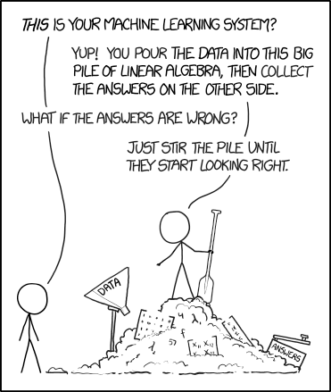
They’re used for
- Representation of data: a structured way to organize and manipulate data, allowing complex datasets to be represented as matrices
- dimensionality reduction: techniques like PCA rely on linear algebra to reduce the number of variables to enhance model efficiency without losing important information
- optimization: gradient descent, the core engine for ML, uses linear algebra to find the minimum of a function.
- Feature engineering: linear transformation and matrix operations create new features from existing data
- similarity measures: embeddings are stored as vectors and are used in recommendation systems and AI chatbots today.
- and many more!
This article will look at some linear algebra concepts, visual explanations, and code examples.
Let’s dive right in!
Code → Deepnote Notebook
Table of contents
Vector
∘ Unit vector
Vector operations
∘ Vector addition
∘ Scalar multiplication
∘ Dot product
Vector space
∘ Null space (kernel)
∘ Span
∘ Basis
∘ Linear Independence
Matrix
∘ Matrices as functions
∘ Linear Transformation
∘ Inverse Matrix
∘ Singular Matrix
∘ Identity matrix.
∘ Diagonal Matrix
∘ Orthogonal matrix
∘ Matrix multiplication
∘ Trace
∘ Determinant
∘ Rank
∘ Eigenvectors and Eigenvalues
Vector

This is the fundamental building block of linear algebra.
There are 3 ways to think of a vector.
The first is the physics perspective: vectors are arrows pointing in space, defined by length and direction. Vectors on a flat plane are 2-dimensional, and those in the space we live in are 3-dimensional.
The second is the computer science perspective: vectors are ordered lists of numbers. The length of this list determines the dimension.
The third is the mathematician’s perspective: vectors can be anything where two vectors are added and multiplied by a number.
Unit vector
A unit vector is a vector with a magnitude of 1. It is often used to represent the direction of a vector without regard to its magnitude.
Vector operations
Vector addition

The addition of two vectors to form a new vector, component-wise.

Scalar multiplication
Scalar multiplication is the multiplication of a vector by a scalar (a number) that results in the vector with the same direction (or opposite if the scalar is negative) as the original vector but with a magnitude that is scaled by the absolute value of the scalar.
Dot product
Formally, it is the product of the Euclidian magnitudes of two vectors and the cosine of the angle between them, reflecting both the length of the vectors and their directional relationship.

Intuitively, think of it as applying the directional growth of one vector to another or “How much push/energy is one vector giving to the other?”. The result is how much stronger we’ve made the original vector (positive, negative, or zero)
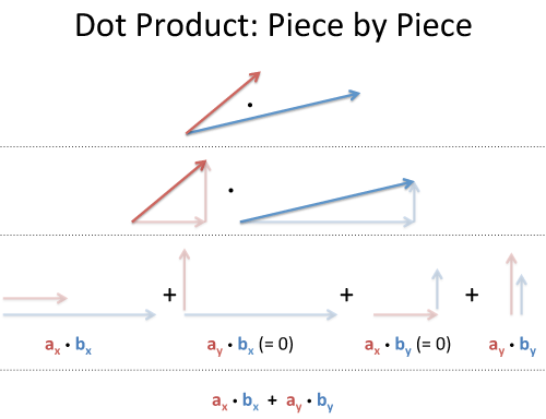
If the dot product is 0, it tells us that the vectors are orthogonal.

A fun analogy by betterexplained
Imagine the red vector is your speed, and the blue vector is the orientation of the boost pad. Larger numbers = more power. The dot product is how much boost you will get.
Using the equation, |a| is your incoming speed, |b| is the max boost, the percentage of boost you get is cos(𝛉), for an overall boost of |a| |b| cos(𝛉)

Vector space
A vector (or linear) space is any collection of vectors that can be added together and multiplied (“scaled”) by numbers, called scalars in this context.
A list of axioms must be satisfied for V to be called a vector space.

Null space (kernel)
The null space is a set of vectors that, when multiplied by the matrix, results in the zero vector.
It represents the solution to the equation Ax = 0, where A is the given matrix.
Imagine a 2d space with two vectors; the null space of a matrix can be visualized as a subspace that collapses these vectors to the origin (zero vector) when multiplied by the matrix.
Span
The set of all possible vectors you can reach given a linear combination of a given pair of vectors, v and w,
av + bw, and let a and b be all real numbers.
For most pairs of vectors, it can reach every point in the 2d vector plane
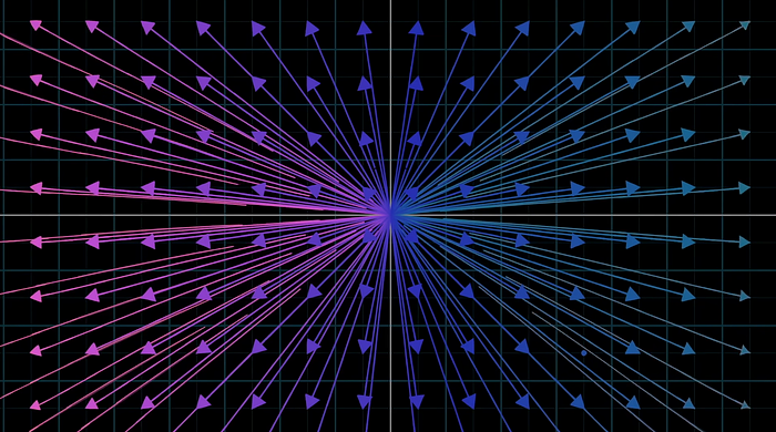
When the two vectors happen to line up, it is limited to the single line that passes through the origin.
The idea of span underlies the idea of basis.
Basis
The basis is a set of linearly independent vectors that span the entire vector space. This means every vector in the vector space can be expressed as a linear combination of the basis vector.
Think of them as the building blocks for all other vectors in the space.
It’s helpful to think of a single vector as an arrow, but for a collection of vectors, think of it as points. Most pairs of basis vectors can span the entire two-dimensional sheet of space.
Linear Independence
A set of vectors is linearly independent if no vectors in the set can be written as a linear combination of others (e.g., a linear combination of x and y would be any expression that forms ax + by, where a and b are constants)
Matrix
Matrices are a way to organize inputs and operations in rows and columns.

Here’s a matrix with 2 rows and 2 columns.
They’re a mathematical tool that can solve problems in a structured manner.
Matrices as functions
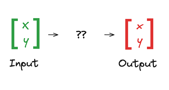
You can think of matrices as functions. Just as a Python function takes input parameters, processes them, and returns output, a matrix transformation transforms input vectors into output vectors through linear transformation.
Linear Transformation
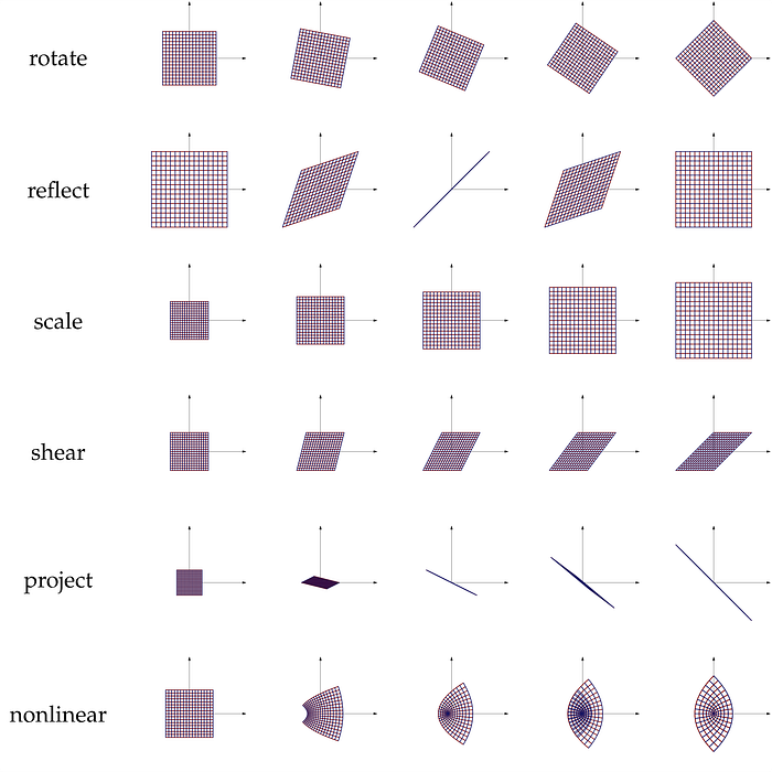
A linear transformation is a mapping V → W between two vector spaces that preserves the operations of vector addition and scalar multiplication.
In practical terms, applying a matrix A to a vector x to get another vector y (via the operation Ax = y) is a linear transformation.
This is used heavily in data science:
- dimensionality reduction: PCA uses linear transformation to map high-dimensional data into lower-dimensional space
- data transformation: normalizing or standardizing a dataset is a linear transformation
- feature engineering: creating new features through combinations of existing ones.
Below are a few forms of matrices
Inverse Matrix
A matrix, when multiplied by its inverse, results in the identity matrix.
Singular Matrix
A singular matrix is a square matrix that does not have an inverse. This is equivalent to saying the matrix’s determinant is zero or its rank is less than its size.
Identity matrix.
The identity matrix is a square matrix with values of one on the diagonals and zero everywhere else. It acts as a multiplicative identity in matrix multiplication, leaving any matrix unchanged by it, just like the number 1.
Diagonal Matrix
A diagonal matrix is a square matrix where all entries outside the main diagonal are zero. It is used in finding eigenvalues, and for calculating the determinant.
Orthogonal matrix
A square matrix with real elements is considered orthogonal if its transpose equals its inverse.
Formally, a matrix A is orthogonal if AᵀA=AAᵀ = I, where I is the identity matrix.
Geometrically, a matrix is orthogonal if its columns and rows are orthogonal unit vectors, a.k.a. they are mutually perpendicular and have a magnitude of 1.
Recall that two vectors are orthogonal if they are perpendicular to each other (90 degrees) and the dot product between them is 0.
Matrix multiplication
You use matrices to perform matrix multiplication.
Here’s a nice visualization from An Intuitive Guide to Linear Algebra

Imagine you’re pouring each input data through each operation.

Here’s an example of this operation.
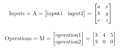
After pouring into the operations, you get this.

The input was a [3 x 2] matrix, and our operation matrix is [2 x 3]; the result is [2 x 3] [3 x 2 ] = [2 x 2].
The size of the input has to match the size of the operation.
Trace
The trace of a matrix is the sum of all its diagonal elements. It is invariant under the change of basis and provides value information about the matrix, i.e., the trace is the sum of the eigenvalues of a matrix.
https://cdn.embedly.com/widgets/media.html?src=https%3A%2F%2Fembed.deepnote.com%2Fa605a3e6-1564-47b2-94e7-842290ba7692%2F3e72bc288b444534881b3da466acf175%2F2543ab7ffd3a437e8172bb1ffe0c5587%3Fheight%3D237.1875&display_name=Deepnote&url=https%3A%2F%2Fembed.deepnote.com%2Fa605a3e6-1564-47b2-94e7-842290ba7692%2F3e72bc288b444534881b3da466acf175%2F2543ab7ffd3a437e8172bb1ffe0c5587%3Fheight%3D237.1875&image=https%3A%2F%2Fdeepnote.com%2Fstatic%2Fthumbnails%2Fmain.png&key=a19fcc184b9711e1b4764040d3dc5c07&type=text%2Fhtml&schema=deepnote
Determinant
Determinant is the size of the output transformation.
If the input was the unit vector (area or volume of 1), the determinant is the size of the transformed area or volume.
Take this matrix, for example. If the area of A was scaled by 6, the determinant of the transformation is 6.


A negative determinant tells us that the entire space was flipped. A transformation of this is like turning a set of paper onto the other side.


Notice how the orientation of the red and green axes was reversed.
A determinant of 0 means the matrix is “destructive” and cannot be reversed. Similar to multiplying by zero, information is lost.
Determinants can tell us whether a matrix is invertible if det(A) is 0, the inverse does not exist; the matrix is singular.
Rank
The maximum number of linearly independent column/row vectors in a matrix. It represents the dimension of the vector space spanned by its rows or columns.
It also tells us the number of output dimensions after a linear transformation.
When the output of a transformation is a single line (it is one-dimensional), we say the transformation has a rank of 1.
If all vectors land on some two-dimensional plane, we say the transformation has a rank of 2.
For a 2×2 matrix, a rank of 2 is the best that it can be. This is known as a full rank. It means the basis vectors can span the entire 2d space and the non-zero determinant.
But for 3×3 matrices, a rank of 2 means it collapsed, but not as much as a rank of 1.
https://cdn.embedly.com/widgets/media.html?src=https%3A%2F%2Fembed.deepnote.com%2Fa605a3e6-1564-47b2-94e7-842290ba7692%2F3e72bc288b444534881b3da466acf175%2F653ad0f4e84b4bfcbb3ce243d51a1373%3Fheight%3D641.4375&display_name=Deepnote&url=https%3A%2F%2Fembed.deepnote.com%2Fa605a3e6-1564-47b2-94e7-842290ba7692%2F3e72bc288b444534881b3da466acf175%2F653ad0f4e84b4bfcbb3ce243d51a1373%3Fheight%3D641.4375&image=https%3A%2F%2Fdeepnote.com%2Fstatic%2Fthumbnails%2Fmain.png&key=a19fcc184b9711e1b4764040d3dc5c07&type=text%2Fhtml&schema=deepnote
Eigenvectors and Eigenvalues
Eigenvectors and eigenvalues represent the “axes” of transformation.
Eigenvectors are inputs that don’t change direction after a linear transformation. Even though the direction doesn’t change, the size might. This size, the amount that the eigenvector is scaled up or down, is the eigenvalue.
Think about when you spin a globe; every location faces a new direction except the poles. Their direction doesn’t change.
Here’s a visual example of eigenvectors.
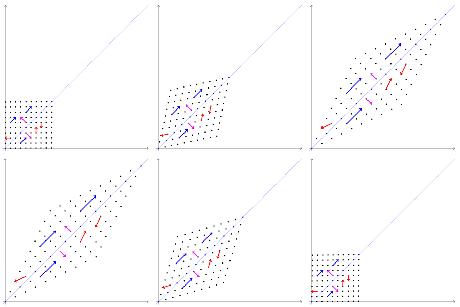
Formally, for a matrix A and a vector v, if Av = λv, then λ is an eigenvalue, and v is an eigenvector of A.
Anther way of saying this is the eigenvectors of a square matrix A are vectors for which matrix multiplication = scalar multiplication.
